Compound Poisson (Spatial) Time Series
Sherman Lo - 2021
Introduction
The compound Poisson distribution was used to model precipitation (Revfeim, 1984; García, 1995; Dunn, 2004; Dzupire, 2018), insurance claims (Jørgensen, 1994; Smyth, 2002) and x-ray images (Whiting, 2002; Elbakri, 2003; Whiting, 2006), the latter was the topic of a PhD thesis (Lo, 2020). The distribution is interesting because it models zero-inflated positive numbers and it is in the exponential family under certain conditions (Jørgensen, 1987). This report covers the compound Poisson and extends it to a time series in the context of precipitation forecasting.
Many materials presented here were copied from (Lo, 2020) which includes further algebra.
The notation used may vary compared to other literature.
Compound Poisson
Define a latent variable \(Z\sim\mathrm{Poisson}(\lambda)\) with probability mass function (p.m.f.) \(\mathbb{P}(Z=z)=\mathrm{e}^{-\lambda}\frac{\lambda^z}{z!}\) for \(z=0,1,2,\ldots\), where \(\lambda>0\) is the Poisson rate parameter. Let \(U_i\) be some independent and identically distributed (i.i.d.) latent random variables for \(i=1,2,3,\ldots\). Let \(Y|Z\) be \[ Y|Z = \sum_{i=1}^{Z}U_i \ . \label{eq:compoundPoisson_X|Y} \] The probability density function (p.d.f.) of \(Y\) can be obtained by marginalising the joint p.d.f. \[ p_Y(y)=\sum_{z=0}^\infty p_{Y|Z}(y|z)\mathbb{P}(Z=z) \quad\text{for }y\geqslant 0 \ . \] It should be noted that \(Y=0\) if and only if \(Z=0\) and this happens with probability \(\mathbb{P}(Z=0)=\mathrm{e}^{-\lambda}\). This implies that \(Y\) has probability mass at zero and probability density for positive numbers which results in the p.d.f. \[ p_Y(y) = \begin{cases} \delta(y) \mathrm{e}^{-\lambda} & \text{ for } y=0 \\ \displaystyle\sum_{z=1}^\infty p_{Y|Z}(y|z)\mathrm{e}^{-\lambda}\dfrac{\lambda^z}{z!} \quad & \text{ for } y>0 \end{cases} \] where \(\delta(y)\) is the Dirac delta function.A special case occurs when \(U_i\sim\mathrm{Gamma}\left(\alpha,\beta\right)\) where \(\alpha>0\) is the gamma shape parameter and \(\beta>0\) is the gamma rate parameter. Then it can be shown that \(Y|Z\sim\mathrm{Gamma}(Z\alpha, \beta)\). The random variable \(Y\) follows the compound Poisson distribution, sometimes called the compound Poisson-Gamma distribution, and is denoted by \(Y\sim\mathrm{CP}(\lambda,\alpha,\beta)\). The p.d.f. is \[ p_Y(y) = \begin{cases} \delta(y) \mathrm{e}^{-\lambda} & \text{ for } y=0 \\ \displaystyle\sum_{z=1}^{\infty}\dfrac{\beta^{z\alpha}}{\Gamma(z\alpha)}y^{z\alpha-1}\mathrm{e}^{-\beta y}\mathrm{e}^{-\lambda}\frac{\lambda^z}{z!} & \text{ for } y>0 \end{cases} \ . \label{eq:compoundPoisson_pdf} \]
Exponential Family
It can be shown that the compound Poisson distribution is in the exponential family for known \(\alpha\) (Jørgensen, 1987). To show this, the compound Poisson distribution was parametrised using the following: \[ p=\frac{2+\alpha}{1+\alpha} \ , \] \[ \mu=\frac{\lambda\alpha}{\beta} \ , \] \[ \phi = \frac{\alpha+1}{\beta^{2-p}(\lambda\alpha)^{p-1}} \ . \] The parameters \(p\), \(\mu\) and \(\phi\) are called the index, mean and dispersion parameters respectively and take the values of \( 1 < p < 2 \), \( \mu> 0 \) and \( \phi > 0 \). It can be shown that the p.m.f. at zero is \[ \mathbb{P}(Y=0) = \exp \left[ -\frac{\mu^{2-p}}{\phi(2-p)} \right] \] and the p.d.f. for \(y>0\) is \[ p_Y(y) = \exp\left[ \frac{1}{\phi} \left( y\frac{\mu^{1-p}}{1-p}-\frac{\mu^{2-p}}{2-p} \right) \right] \frac{1}{y} \sum_{z=1}^{\infty}W_z(y,p,\phi) \] where \[ W_z = W_z(y,p,\phi)=\frac{y^{z\alpha}}{\phi^{z(1+\alpha)}(p-1)^{z\alpha}(2-p)^zz!\Gamma(z\alpha)} \ . \] This is in the form of a distribution in the dispersive exponential family (Nelder and Wedderburn, 1972; Nelder and Baker, 1972; McCullagh, 1984) \[ p_Y(y)=\dfrac{\exp\left(y\theta\right)g(y)}{Z(\theta)} \] where \(Z(\theta)\) is the partition function and \(\theta\) is the natural parameter. For the compound-Poisson, the natural parameter is \[ \theta = \theta(\mu) = \dfrac{\mu^{1-p}}{\phi(1-p)} \label{eq:appendix_cp_naturalParameter} \] and the partition function is \[ Z = Z(\mu) = \exp\left[ \frac{\mu^{2-p}}{\phi(2-p)} \right] \] or in terms of the natural parameter \[ Z = Z(\theta) = \exp\left[ \phi^{\frac{1}{1-p}} \cdot \theta^{\frac{2-p}{1-p}} \cdot \dfrac{ (1-p)^{\frac{2-p}{1-p}} }{ 2-p } \right] \ . \]
The partition function has some useful properties such as \[ \mathbb{E}[Y] = \dfrac{\partial \ln Z}{\partial \theta} \] and \[ \mathbb{V}\mathrm{ar}\left[Y\right] = \dfrac{\partial^2\ln Z}{\partial \theta^2} \ . \label{eq:appendix_variancePartitionFunction} \] Thus it can be shown that \[ \mathbb{E}[Y] = \mu \] and \[ \mathbb{V}\mathrm{ar}[Y] = \phi \mu^p \] which shows that the compound Poisson distribution is in the Tweedie dispersion exponential family with \( 1 < p < 2 \), making it suitable for generalised linear models.
Parameter Estimation
Suppose \(Y_i\sim\mathrm{CP}(\lambda, \alpha, \beta)\) for \(i=1,2,\ldots,N\) and i.i.d. with the following observations \(y_1, y_2, \ldots, y_N\) respectively. It is possible to estimate the parameters \(\lambda, \alpha\) and \(\beta\) numerically using using maximum likelihood where the log likelihood is \(\ln L=\sum_{i=1}^N\ln p_Y(y_i)\). When evaluating the log likelihood, thus the p.d.f. as well, the infinite sum \(\sum_{z=1}^{\infty}W_z(y,p,\phi)\) can be calculated approximately by summing over a finite number of large terms (Dunn, 2005). One method to maximise the likelihood is the EM algorithm (Dempster, 1977) by iteratively estimating \(Z_i|Y_i,\lambda,\alpha,\beta\) for \(i=1,2,\ldots,N\) followed by estimating \(\lambda,\alpha,\beta|Z_1,Y_1,Z_2,Y_2,\ldots,Z_N,Y_N\). This was explored in (Lo, 2020) but required numerous approximations.
Method of moments estimators does exist (Withers and Nadarajah, 2011).
For known \(p\) or \(\alpha\), the compound Poisson is in the exponential family so parameter estimation can be done via the generalised linear model framework (see the R package cpglm) (Zhang, 2013). Estimating \(p\) is difficult and various methods were discussed (Zhang, 2013). One way is to estimate \(\mu\) and \(\phi\) on a grid of \(p\)'s and then select the \(p\) which maximises the likelihood (Dunn, 2005).
Time Series
In the precipitation forecasting problem, a time series for the model fields \(x_1, x_2, \ldots, x_T\) is given. The objective is to use the model fields as explanatory variables for the time series of the precipitation \(Y_1, Y_2, \ldots, Y_T\). The time series can be simplified by fixing \(\alpha\) so that the distribution of the time series is in the exponential family. Such a simplification can introduce auto-correlation behaviour using the generalised autoregressive moving-average (GARMA) model (Benjamin, 1998).
To study the compound Poisson in the exponential family, the compound Poisson is to be parameterised as \[ Y_t \sim \mathrm{CP}\left( \dfrac{\mu_t^{2-p}}{\phi(2-p)}, \alpha, \dfrac{1}{\phi(p-1)\mu_t^{p-1}} \right) \] so that the index parameter, \(p\), and the dispersion parameter, \(\phi\), are fixed. The mean parameters, \(\mu_1, \mu_2, \ldots, \mu_T\), can be made as a function of the model fields \[ \eta_t=g(\mu_t) \] where \(g(\mu)\) is some link function and \(\eta_t=\eta(x_t)\) is the systematic component. An example of a systematic component is a basic linear relationship \[ \eta_t=x_t \beta \] where \(\beta\) is the regression parameter.
The choice of the link function \(g(\mu_t)\) is left as a free choice. But because a compound Poisson random variable can take non-negative values, it is recommended that the link function has a domain of \(0 < \mu < \infty\) and range \(-\infty < g(\mu_t) < \infty\). An example would be the log link function \[ g(\mu_t)=\ln(\mu_t) \ . \]
The GARMA model (Benjamin, 1998) include autoregressive and moving-average terms \[ \eta_t=x_t \beta + \sum_{i=1:t>i}^r \phi_i \left(g(y_{t-i})-x_{t-i}\beta\right) + \sum_{j=1:t>j}^s\theta_j\left( g(y_{t-j})-\eta_{t-j} \right) \] where \(\phi_1,\phi_2,\ldots,\phi_r\) are autoregressive (AR) parameters and \(\theta_1,\theta_2,\ldots,\theta_s\) are moving-average (MA) parameters. (Benjamin 1998) used the Normal, Gamma and Poisson distributions as examples of distributions from the exponential family. However, when used with the log link function, the AR and MA components for GARMA are not suitable for the compound Poisson because the AR and MA components would take values of \(-\infty\) when \(y_{t-1}=0\), i.e. when it has not rained on the previous day. A way around it is to replace \(y_t\) with \(y_t^*\) such that \[ \eta_t = x_t \beta + \sum_{i=1:t>i}^r \phi_i \left(g(y_{t-i}^*)-x_{t-i}\beta\right) \\+ \sum_{j=1:t>j}^s\theta_j\left( g(y_{t-j}^*)-\eta_{t-j} \right) \] where \[ y_t^*=\max(y_t, c) \] and \(c\) is a small positive number (Benjamin, 1998). This allows the evaluation of \(g(y_{t-i}^*)\) to be possible for \(y_{t-i}=0\).
Another option is to remove the AR element and consider positive \(\theta_j\). This can be studied by considering one MA term \[ \eta_t = x_t \beta + \theta_1\left( g(y_{t-1})-\eta_{t-1} \right) \] and to investigate the limiting scenarios. Consider a finite \(\eta_{t-1}\) which implies a finite \(\mu_{t-1}\) and a non-zero probability that \(Y_{t-1}=0\). If \(y_{t-1}=0\) was observed, then this would cause \(g(y_{t-1})\rightarrow -\infty\), \(\eta_{t}\rightarrow -\infty\) and \(\mu_t\rightarrow 0\). In this limiting case, \(Y_t=0\) with probability one. For the following day, the systematic component is \( \eta_{t+1} = x_{t+1} \beta + \theta_1\left( g(y_{t})-\eta_{t} \right) \). Because \(y_t=0\), \(g(y_t)\rightarrow - \infty\) and \(\eta_t\rightarrow - \infty\), it could be suggested that \(g(y_t)-\eta_t=0\) which would make is possible for \(\eta_{t+1}\) to be finite. Then for non zero \(\theta_1,\theta_2,\ldots,\theta_s\), another version of the systematic component is \[ \eta_t = x_t\beta + \sum_{j=1:t>j}^s\theta_j\Theta_{t-j} \] where \[ \Theta_{t} = \begin{cases} -\infty & \text{if }y_t=0\text{ and } \mu_t\neq 0 \\ 0 & \text{if }y_t=0\text{ and } \mu_t= 0 \\ g(y_{t})-\eta_{t} & \text{otherwise} \end{cases} \ . \] This version may be too restrictive, for example, dry days can only occur on consecutive days.


There may be a possibility to relax the fixed \(p\) and \(\phi\) assumption but it shall not be discussed here.
Discussion
The GARMA model for the compound Poisson is unsuitable to model precipitation because the assumptions required produce unrealistic results, e.g. dry days can only occur on consecutive days. This stems from the fact that the log link function is applied to realisations of the compound Poisson, \(g(y_t)\), in the systematic component and problems arise on dry days, \(y_t=0\).
Methods for parameter fitting, model selection and forecasting are omitted but important when applying to precipitation forecasting. Model selection investigates how many AR and MA terms to use and what model fields to include in the systematic component. For model fitting, numerical methods would be required to maximise a likelihood or to study a posterior distribution using methods such as gradient descent or Markov chains using Monte Carlo (Brooks, 2011).
Any stationarity assumptions were not investigated here but it has been demonstrated that the GARMA model for the compound Poisson is quite restrictive.
The model can be further generalised, for example, the systematic component could be \(\eta_t=f_\beta(x_t)\) where \(f_\beta(x_t)\) is a neural network parameterised by \(\beta\) to allow for non-linear relationships.
Other distributions to model precipitation were studied, for example, using a mixture of zero mass and Gamma distributions (Holsclaw, 2017; Bertolacci, 2019). It could be argued that the compound Poisson has some strengths, for example, the occurrences of rain can be modelled as well. High winds could contribute to higher occurrences of rain by moving scattered rain clouds across the country.
Another advantage is that the compound Poisson distribution is in the exponential family which could lead to simpler mathematics and the potential to use existing methods.
Spatial Forecasting
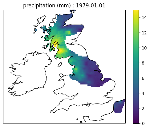
Forecasting precipitation becomes interesting when forecasting multiple locations on a grid. Figure 2 shows observed precipitation from the E-obs dataset (Cornes et al., 2019). Realistically, rain clouds form shapes and a smooth boundary between zero and positive precipitation can be seen in the observed data. Spatial forecasting should aim to replicate such spatial structure if realism is important.
Suppose each point on the grid has coordinates \(\mathbf{r}_1,\mathbf{r}_2,\ldots,\mathbf{r}_M\). A simple strategy to model multiple locations is to fit the model to each location independently; each location will have different inferred parameters which can be learnt independently. Another option is to put a Gaussian process prior (Williams and Rasmussen, 1996) on the parameters to allow them to be spatially smooth. However, these methods are not realistic because the resulting model does not form rain clouds. Even if each location has the same parameters, the realised precipitation is not spatially smooth. Imagine the entire grid has the state space \(\lambda_t=1\), the realised grid of \(Z_t\)'s would be wet and drypoints scattered randomly across the grid; this is not characteristic of rain clouds.
Rain clouds can be formed using a graphical model for the Poisson-element (Yang et al., 2013). Consider a day \(t\) and let \(Z_{\mathbf{r}_1}, Z_{\mathbf{r}_2}, \ldots, Z_{\mathbf{r}_M}\) be the latent Poisson variable with respective rate parameters \(\lambda_{\mathbf{r}_1}, \lambda_{\mathbf{r}_2}, \ldots, \lambda_{\mathbf{r}_M}\) for the \(M\) grid points. Let \(Q(\mathbf{r}_i)\) be a collection of four coordinates which neighbours \(\mathbf{r}_i\). The graphical model should persuade \(Z_{\mathbf{r}_i}\) to take the same, or similar, value as \(Z_\mathbf{s}\) for \(\mathbf{s}\in Q(\mathbf{r}_i)\) to form rain clouds. This can be done by adjusting the conditional p.m.f. of \(Z_{\mathbf{r}_i}\) to \[ \mathbb{P}(Z_{\mathbf{r}_i} = z| Z_\mathbf{s} : \mathbf{s}\in Q(\mathbf{r}_i)) \propto \exp\left[ z\ln \lambda_{\mathbf{r}_i} - \ln{z!} - \sum_{\mathbf{s}\in Q(\mathbf{r}_i)} \gamma \left(z - Z_\mathbf{s}\right)^2 \right] \] where \(\gamma\) is the interaction parameter. The interaction term decreases the p.m.f. for values of \(z\) which deviates too much from it neighbours which should hopefully encourages the forming of rain clouds. However, as with many graphical models, inference can be computationally intensive, let alone for \(T\) lots of graphical models to form a spatial forecast.
References
- Benjamin, M. A., Rigby, R. A., and Stasinopoulos, M. D. (1998). Modelling exponential family time series data. In Statistical Modelling: Proceedings of the 13th International Workshop on Stastical Modelling. Citeseer.
- Bertolacci, M., Cripps, E., Rosen, O., Lau, J. W., Cripps, S., et al. (2019). Climate inference on daily rainfall across the Australian continent, 1876-2015. The Annals of Applied Statistics, 13(2):683-712.
- Brooks, S., Gelman, A., Jones, G. L., and Meng, X.-L. (2011). Handbook of Markov chain Monte Carlo. CRC Press.
- Cornes, R., van der Schrier, G., van den Besselaar, E., and Jones, P. (2019). An ensemble version of the e-obs temperature and precipitation datasets: version 21.0e.
- Dempster, A. P., Laird, N. M., and Rubin, D. B. (1977). Maximum likelihood from incomplete data via the EM algorithm. Journal of the Royal Statistical Society: Series B (Methodological), 39(1):1-38.
- Dunn, P. K. (2004). Occurrence and quantity of precipitation can be modelled simultaneously. International Journal of Climatology: A Journal of the Royal Meteorological Society, 24(10):1231-1239.
- Dunn, P. K. and Smyth, G. K. (2005). Series evaluation of Tweedie exponential dispersion model densities. Statistics and Computing, 15(4):267-280.
- Dzupire, N. C., Ngare, P., and Odongo, L. (2018). A Poisson-gamma model for zero inflated rainfall data. Journal of Probability and Statistics, 2018.
- Elbakri, I. A. and Fessler, J. A. (2003). Efficient and accurate likelihood for iterative image reconstruction in x-ray computed tomography. In Proceedings of SPIE Medical Imaging: Image Processing, volume 5032.
- García, J., Marroquin, A., Garrido, J., and Mateos, V. (1995). Analysis of daily rainfall processes in lower extremadura (Spain) and homogenization of the data. Theoretical and Applied Climatology, 51(1):75-87.
- Holsclaw, T., Greene, A. M., Robertson, A. W., Smyth, P., et al. (2017). Bayesian nonhomogeneous markov models via pólya-gamma data augmentation with applications to rainfall modeling. The Annals of Applied Statistics, 11(1):393-426.
- Jørgensen, B. (1987). Exponential dispersion models. Journal of the Royal Statistical Society: Series B (Methodological), pages 127-162.
- Jørgensen, B. and Paes De Souza, M. C. (1994). Fitting Tweedie's compound Poisson model to insurance claims data. Scandinavian Actuarial Journal, 1994(1):69-93.
- Lo, S. E. (2020). Characterisation of Computed Tomography Noise in Projection Space with Applications to Additive Manufacturing. PhD thesis, University of Warwick.
- McCullagh, P. (1984). Generalized linear models. European Journal of Opera- tional Research, 16(3):285-292.
- Nelder, J. A. and Baker, R. J. (1972). Generalized linear models. Encyclopedia of Statistical Sciences.
- Nelder, J. A. and Wedderburn, R. (1972). Generalized linear models. Journal of the Royal Statistical Society: Series A (General), 135(3):370-384.
- Revfeim, K. J. A. (1984). An initial model of the relationship between rainfall events and daily rainfalls. Journal of Hydrology, 75(1):357-364.
- Smyth, G. K. and Jørgensen, B. (2002). Fitting Tweedie's compound Poisson model to insurance claims data: Dispersion modelling. Astin Bulletin, 32(01):143-157.
- Whiting, B. R. (2002). Signal statistics in x-ray computed tomography. In Proceedings of SPIE Medical Imaging: Physics of Medical Imaging, volume 4682.
- Whiting, B. R., Massoumzadeh, P., Earl, O. A., O'Sullivan, J. A., Snyder, D. L., and Williamson, J. F. (2006). Properties of preprocessed sinogram data in x-ray computed tomography. Medical Physics, 33(9):3290-3303.
- Williams, C. K. I. and Rasmussen, C. E. (1996). Gaussian processes for regression. In Proceedings of Advances in Neural Information Processing Systems, pages 514-520.
- Withers, C. and Nadarajah, S. (2011). On the compound Poisson-gamma distribution. Kybernetika, 47(1):15-37.
- Yang, E., Ravikumar, P. K., Allen, G. I., and Liu, Z. (2013). On Poisson graphical models. In Proceedings of Advances in Neural Information Processing Systems, pages 1718-1726.
- Zhang, Y. (2013). Likelihood-based and Bayesian methods for Tweedie compound Poisson linear mixed models. Statistics and Computing, 23(6):743-757.